
Introduction
Hash tables are a fundamental data structure used in computer science for fast data retrieval. They store key-value pairs and offer remarkable efficiency in searching for a value associated with a given key.
We previously learned about linked lists. We mentioned that one main advantages of them is that we can efficiently and dynamically add or remove elements to/from the front of the list in O(1) runtime complexity. We know that arrays are very good when it comes to element access, which we can do in constant O(1) runtime complexity.
a Hash Table is a data structure that stores data in a way that benefits from the best of both worlds, leveraging the advantages of both the array and the linked list.
In this article we are going to show the fundamentals of the hash table, by showing a hashing technique called Chain Hashing.
Structure
A hash table that uses chain hashing is built of 2 components:
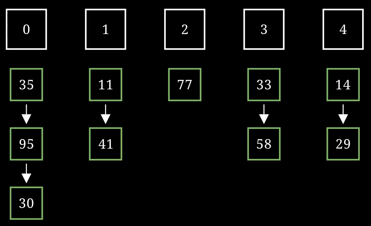
- An array of buckets – Each bucket is the head of a linked list.
- A hash function h(x) – The function gets a key of an element and returns a number. The number is the index of the “bucket” that the element should belong to.
Each cell in the array has a linked list that can hold multiple elements. This makes sure we can handle collisions.
Operations
Adding an element
- First, the key associated with the value to be added is passed through a hash function, which computes an index based on the key’s characteristics. This index determines which bucket in the hash table array the key-value pair will be placed in.
- If the bucket is empty, the key-value pair is inserted directly, becoming the head of a new linked list at that bucket. if the bucket already contains one or more key-value pairs (a situation indicating a collision), the new pair is added to the linked list at that bucket. This can be done by inserting the new pair at the beginning, making it the new head (for efficiency), or at the end of the list, depending on the implementation’s design.
Here is a simple video demonstrating additions to an empty hash table (that has an array of size 5), and uses a single hash function that calculates the key modulo the size of the array i=h(x) \mod n, to get an index:
Searching for an element
- Just like the previous case, we first calculate the index of the bucket by passing the key to be added into the hash function. This gives us the relevant linked list.
- Iterate element by element over the linked list and see if you can find the wanted value.
Here is a video that demonstrates the search operation over the hash table, by again using a hash function that calculates the modulo with the array size in order to get the index:
Removal of an element
- Just like previous cases, we first find the bucket in which the element should be removed from by running the hash function.
- We go over the relevant list to see if we can find the element to be removed
- The removal is a standard removal operation from a linked list, which updates the pointer of the previous node, to point to the node after the one that was deleted.
Runtime Complexity
| Operation | Average Case Complexity | Worst Case Complexity |
|---|---|---|
| Insertion | O(1) | O(n) |
| Search | O(1) | O(n) |
| Deletion | O(1) | O(n) |
The efficiency of the operations is achieved by two assumptions about the hash function:
- The hash function is deterministic – The hash function needs to be deterministic to make sure we get the same index when searching for an element every time. Failing to do so will make us think an element does not exist / miss it when looking for it.
- The hash function evenly distributes the input in the array – A good hash function will make sure the “load factor” of every list is not too high. This makes sure the length of the lists we are searching on is never too long.
Average-Case Complexity
- Insertion: O(1). Inserting a new key-value pair is typically a constant-time operation. The hash function computes the index for the key in constant time, and the pair is added to the corresponding bucket. In the case of chaining, this means appending the pair to a linked list, which is an O(1) operation if the insertion happens at the head of the list.
- Search: O(1) on average. The hash function quickly locates the bucket (constant time), but finding the exact key-value pair requires traversing the chain. However, if the hash function distributes keys uniformly and the load factor (number of entries divided by the number of buckets) is kept low, the length of the list is small, and this operation remains efficient.
- Deletion: O(1) on average, for similar reasons as search. Once the bucket is found, the linked list must be traversed to find and remove the key-value pair. Like search, this operation is efficient when the list is kept small.
Worst-Case Complexity
The worst-case scenarios for hash table operations occur when the hash function does not distribute keys evenly across the buckets, leading to a high load factor or clustering at certain indices. In such cases, many or all keys could hash to the same bucket, and the complexities become:
- Insertion: O(n), where n is the number of elements in the hash table. This happens if every key hashes to the same bucket, making the insertion operation equivalent to appending an item to a linked list of length n.
- Search: O(n), for the same reason as insertion. If all keys are in the same bucket, looking up a key requires traversing a linked list of all n elements.
- Deletion: O(n), because finding and removing a key-value pair would involve traversing the entire list if all elements hash to the same bucket.
Advantages of Hash Tables over Linked Lists
Faster Search, Insert, and Delete Operations: The most significant advantage of hash tables is their ability to perform search, insert, and delete operations in constant time, O(1) under optimal conditions. In contrast, linked lists require O(n) time for search and delete operations, as you may need to traverse the list to find the item.
Direct Access: Hash tables provide direct access to data through keys, making it unnecessary to traverse the structure to find an item, unlike linked lists where traversal from the head to the desired node is often required.
Advantages of Hash Tables over Arrays
Dynamic Sizing: Arrays have a fixed size, meaning you must know the maximum number of elements in advance. While dynamic arrays and array lists can resize, resizing is a costly operation that involves creating a new, larger array and copying all elements to it. Hash tables, especially those designed with dynamic resizing in mind, handle resizing more gracefully, allowing the data structure to grow as needed without significant performance degradation.
Key-Value Storage: Hash tables inherently store data as key-value pairs, making them ideal for scenarios where associative data storage is required. This is a stark contrast to arrays, which only store values and require additional mechanisms to associate keys with those values.